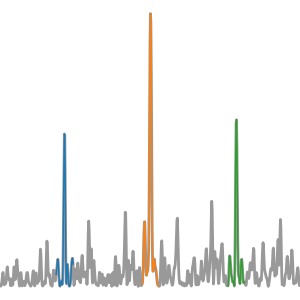
Lomb-Scargle periodogram¶

The Lomb-Scargle periodogram ([Barning1963], [Vanicek1969], [Scargle1982], [Lomb1976]) is one of the best known and most popular period finding algorithms used in astrononomy. If you would like to learn more about least-squares methods for periodic signals, see the review article by [VanderPlas2017].

The LS periodogram is a least-squares estimator for the following model

\[\hat{y}(t|\omega, \theta) = \theta_1\cos{\omega t} + \theta_2\sin{\omega t}\]

and it is equivalent to the Discrete Fourier Transform in the regularly-sampled limit. For irregularly sampled data, LS is a maximum likelihood estimator for the parameters \(\theta\) in the case where the noise is Gaussian. The periodogram has many normalizations in the literature, but cuvarbase adopts

\[P(\omega) = \frac{\chi^2_0 - \chi^2(\omega)}{\chi^2_0}\]

where

\[\chi^2(\omega) = \sum_i \left(\frac{y_i - \hat{y}(t_i|\omega, \theta)}{\sigma_i}\right)^2\]

is the goodness-of-fit statistic for the optimal parameters \(\theta\) and

\[\chi^2_0 = \sum_i \left(\frac{y_i - \bar{y}}{\sigma_i}\right)^2\]

is the goodness-of-fit statistic for a constant fit, and \(\bar{y}\) is the weighted mean,

\[\bar{y} = \sum_i w_i y_i\]

where \(w_i \propto 1/\sigma_i^2\) and \(\sum_iw_i = 1\).

The closed form of the periodogram is given by

\[P(\omega) = \frac{1}{\chi^2_0}\left(\frac{YC_{\tau}^2}{CC_{\tau}} + \frac{YS_{\tau}^2}{SS_{\tau}}\right)\]

Where

\[ \begin{align}\begin{aligned}\begin{split}YC_{\tau} &= \sum_i w_iy_i\cos{\omega (t_i - \tau)}\\\end{split}\\\begin{split}YS_{\tau} &= \sum_i w_iy_i\sin{\omega (t_i - \tau)}\\\end{split}\\\begin{split}CC_{\tau} &= \sum_i w_i\cos^2{\omega (t_i - \tau)}\\\end{split}\\\begin{split}SS_{\tau} &= \sum_i w_i\sin^2{\omega (t_i - \tau)}\\\end{split}\\\tan{2\omega\tau} &= \frac{\sum_i w_i \sin{2\omega t_i}}{\sum_i w_i \sin{2\omega t_i}}\end{aligned}\end{align} \]

For the original formulation of the Lomb-Scargle periodogram without the constant offset term.

Adding a constant offset¶

Lomb-Scargle can be extended in many ways, most commonly to include a constant offset [ZK2009].

\[\hat{y}^{\rm GLS}(t|\omega, \theta) = \theta_1\cos{\omega t} + \theta_2\sin{\omega t} + \theta_3\]

This protects against cases where the mean of the data does not correspond with the mean of the underlying signal, as is usually the case with sparsely sampled data or for signals with large amplitudes that become too bright or dim to be observed during part of the signal phase.

With the constant offset term, the closed-form solution to \(P(\omega)\) is the same, but the terms are slightly different. Derivations of this are in [ZK2009].

Getting \(\mathcal{O}(N\log N)\) performance¶

The secret to Lomb-Scargle’s speed lies in the fact that computing it requires evaluating sums that, for regularly-spaced data, can be evaluated with the fast Fourier transform (FFT), which scales as \(\mathcal{O}(N_f\log N_f)\) where \(N_f\) is the number of frequencies. For irregularly spaced data, however, we can employ tricks to get to this scaling.

We can “extirpolate” the data with Legendre polynomials to a regular grid and then perform the FFT [PressRybicki1989], or,
We can use the non-equispaced fast Fourier transform (NFFT) [DuttRokhlin1993], which is tailor made for this exact problem.

The latter was shown by [Leroy2012] to give roughly an order-of-magnitude speed improvement over the [PressRybicki1989] method, with the added benefit that the NFFT is a rigorous extension of the FFT and has proven error bounds.

It’s worth mentioning the [Townsend2010] CUDA implementation of Lomb-Scargle, however this uses the \(\mathcal{O}(N_{\rm obs}N_f)\) “naive” implementation of LS without any FFT’s.

Estimating significance¶

See [Baluev2008] for more information (TODO.)

Example: Basic¶

import skcuda.fft
import cuvarbase.lombscargle as gls
import numpy as np
import matplotlib.pyplot as plt


t = np.sort(np.random.rand(300))
y = 1 + np.cos(2 * np.pi * 100 * t - 0.1)
dy = 0.1 * np.ones_like(y)
y += dy * np.random.randn(len(t))

# Set up LombScargleAsyncProcess (compilation, etc.)
proc = gls.LombScargleAsyncProcess()

# Run on single lightcurve
result = proc.run([(t, y, dy)])

# Synchronize all cuda streams
proc.finish()

# Read result!
freqs, ls_power = result[0]

############
# Plotting #
############

f, ax = plt.subplots()
ax.set_xscale('log')

ax.plot(freqs, ls_power)
ax.set_xlabel('Frequency')
ax.set_ylabel('Lomb-Scargle')
plt.show()

(Source code)

Example: Batches of lightcurves¶

import skcuda.fft
import cuvarbase.lombscargle as gls
import numpy as np
import matplotlib.pyplot as plt

nlcs = 9

def lightcurve(freq=100, ndata=300):
        t = np.sort(np.random.rand(ndata))
        y = 1 + np.cos(2 * np.pi * freq * t - 0.1)
        dy = 0.1 * np.ones_like(y)
        y += dy * np.random.randn(len(t))
        return t, y, dy

freqs = 200 * np.random.rand(nlcs)
data = [lightcurve(freq=freq) for freq in freqs]

# Set up LombScargleAsyncProcess (compilation, etc.)
proc = gls.LombScargleAsyncProcess()

# Run on batch of lightcurves
results = proc.batched_run_const_nfreq(data)

# Synchronize all cuda streams
proc.finish()

############
# Plotting #
############
max_n_cols = 4
ncols = max([1, min([int(np.sqrt(nlcs)), max_n_cols])])
nrows = int(np.ceil(float(nlcs) / ncols))
f, axes = plt.subplots(nrows, ncols,
                       figsize=(3 * ncols, 3 * nrows))

for (frqs, ls_power), ax, freq in zip(results,
                                      np.ravel(axes),
                                      freqs):
        ax.set_xscale('log')
        ax.plot(frqs, ls_power)
        ax.axvline(freq, ls=':', color='r')

f.text(0.05, 0.5, "Lomb-Scargle", rotation=90,
       va='center', ha='right', fontsize=20)
f.text(0.5, 0.05, "Frequency",
       va='top', ha='center', fontsize=20)


for i, ax in enumerate(np.ravel(axes)):
        if i >= nlcs:
                ax.axis('off')
f.tight_layout()
f.subplots_adjust(left=0.1, bottom=0.1)
plt.show()