Box least squares (BLS) periodogram¶

The box-least squares periodogram [BLS] searches for the periodic dips in brightness that occur when, e.g., a planet passes in front of its host star. The algorithm fits a boxcar function to the data. The parameters used are

q: the transit duration as a fraction of the period \(t_{\rm trans} / P\)
phi0: the phase offset of the transit (from 0)
delta: the difference between the out-of-transit brightness and the brightness during transit
y0: The out-of-transit brightness

(Source code)

Using `cuvarbase` BLS¶

import cuvarbase.bls as bls
import numpy as np
import matplotlib.pyplot as plt


def phase(t, freq, phi0=0.):
    phi = (t * freq - phi0)
    phi -= np.floor(phi)

    return phi


def transit_model(t, freq, y0=0.0, delta=1., q=0.01, phi0=0.5):
    phi = phase(t, freq, phi0=phi0)
    transit = phi < q

    y = y0 * np.ones_like(t)
    y[transit] -= delta
    return y


def data(ndata=100, baseline=1, freq=10, sigma=1., **kwargs):
    t = baseline * np.sort(np.random.rand(ndata))
    y = transit_model(t, freq, **kwargs)
    dy = sigma * np.ones_like(t)

    y += dy * np.random.randn(len(t))

    return t, y, dy


def plot_bls_model(ax, y0, delta, q, phi0, **kwargs):
    phi_plot = np.linspace(0, 1, 50./q)
    y_plot = transit_model(phi_plot, 1., y0=y0,
                           delta=delta, q=q, phi0=phi0)

    ax.plot(phi_plot, y_plot, **kwargs)


def plot_bls_sol(ax, t, y, dy, freq, q, phi0, **kwargs):
    w = np.power(dy, -2)
    w /= sum(w)

    phi = phase(t, freq, phi0=phi0)
    transit = phi < q

    def ybar(mask):
        return np.dot(w[mask], y[mask]) / sum(w[mask])

    y0 = ybar(~transit)
    delta = y0 - ybar(transit)

    ax.scatter((phi[~transit] + phi0) % 1.0, y[~transit],
               c='k', s=1, alpha=0.5)
    ax.scatter((phi[transit] + phi0) % 1.0, y[transit],
               c='r', s=1, alpha=0.5)
    plot_bls_model(ax, y0, delta, q, phi0, **kwargs)

    ax.set_xlim(0, 1)
    ax.set_xlabel('$\phi$ ($f = %.3f$)' % (freq))
    ax.set_ylabel('$y$')

# set the transit parameters
transit_kwargs = dict(freq=0.1,
                      q=0.1,
                      y0=10.,
                      sigma=0.002,
                      delta=0.05,
                      phi0=0.5)

# generate data with a transit
t, y, dy = data(ndata=300,
                baseline=365.,
                **transit_kwargs)

# set up search parameters
search_params = dict(qmin=1e-2,
                     qmax=0.5,

                     # The logarithmic spacing of q
                     dlogq=0.1,

                     # Number of overlapping phase bins
                     # to use for finding the best phi0
                     noverlap=3)

# derive baseline from the data for consistency
baseline = max(t) - min(t)

# df ~ qmin / baseline
df = search_params['qmin'] / baseline
fmin = 2. / baseline
fmax = 2.

nf = int(np.ceil((fmax - fmin) / df))
freqs = fmin + df * np.arange(nf)

bls_power, sols = bls.eebls_gpu(t, y, dy, freqs,
                                **search_params)

# best BLS fit
q_best, phi0_best = sols[np.argmax(bls_power)]
f_best = freqs[np.argmax(bls_power)]

# Plot results
f, (ax_bls, ax_true, ax_best) = plt.subplots(1, 3, figsize=(9, 3))

# Periodogram
ax_bls.plot(freqs, bls_power)
ax_bls.axvline(transit_kwargs['freq'],
               ls=':', color='k', label="$f_0$")
ax_bls.axvline(f_best, ls=':', color='r',
               label='BLS $f_{\\rm best}$')
ax_bls.set_xlabel('freq.')
ax_bls.set_ylabel('BLS power')

# True solution
plot_bls_sol(ax_true, t, y, dy,
             transit_kwargs['freq'],
             transit_kwargs['q'],
             transit_kwargs['phi0'])

# Best-fit solution
plot_bls_sol(ax_best, t, y, dy,
             f_best, q_best, phi0_best)


ax_true.set_title("True parameters")
ax_best.set_title("Best BLS parameters")

f.tight_layout()
plt.show()

(Source code)

A shortcut: assuming orbital mechanics¶

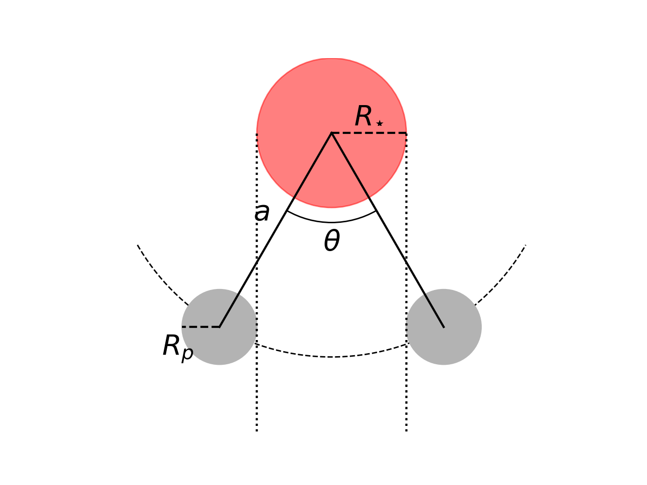
If you assume \(R_p\ll R_{\star}\), \(M_p\ll M_{\star}\), \(L_p\ll L_{\star}\), and \(e\ll 1\), where \(e\) is the ellipticity of the planetary orbit, \(L\) is the luminosity, \(R\) is the radius, and \(M\) mass, you can eliminate a free parameter.

This is because the orbital period obeys Kepler’s third law,

\[P^2 \approx \frac{4\pi^2a^3}{G(M_p + M_{\star})}\]

(Source code, png, hires.png, pdf)

The angle of the transit is

\[\theta = 2{\rm arcsin}\left(\frac{R_p + R_{\star}}{a}\right)\]

and \(q\) is therefore \(\theta / (2\pi)\). Thus we have a relation between \(q\) and the period \(P\)

\[\sin{\pi q} = (R_p + R_{\star})\left(\frac{4\pi^2}{P^2 G(M_p + M_{\star})}\right)^{1/3}\]

By incorporating the fact that

\[R_{\star} = \left(\frac{3}{4\pi\rho_{\star}}\right)^{1/3}M_{\star}^{1/3}\]

where \(\rho_{\star}\) is the average stellar density of the host star, we can write

\[\sin{\pi q} = \frac{(1 + r)}{(1 + m)^{1/3}} \left(\frac{3\pi}{G\rho_{\star}}\right)^{1/3} P^{-2/3}\]

where \(r = R_p / R_{\star}\) and \(m = M_p / M_{\star}\). We can get rid of the constant factors and convert this to more intuitive units to obtain

\[\sin{\pi q} \approx 0.238 (1 + r - \frac{m}{3} + \dots{}) \left(\frac{\rho_{\star}}{\rho_{\odot}}\right)^{-1/3} \left(\frac{P}{\rm day}\right)^{-2/3}\]

where here we’ve expanded \((1 + r) / (1 + m)^{1/3}\) to first order in \(r\) and \(m\).

Using the Keplerian assumption in `cuvarbase`¶

import cuvarbase.bls as bls
import numpy as np
import matplotlib.pyplot as plt


def phase(t, freq, phi0=0.):
    phi = (t * freq - phi0)
    phi -= np.floor(phi)

    return phi


def transit_model(t, freq, y0=0.0, delta=1., q=0.01, phi0=0.5):
    phi = phase(t, freq, phi0=phi0)
    transit = phi < q

    y = y0 * np.ones_like(t)
    y[transit] -= delta
    return y


def data(ndata=100, baseline=1, freq=10, sigma=1., **kwargs):
    t = baseline * np.sort(np.random.rand(ndata))
    y = transit_model(t, freq, **kwargs)
    dy = sigma * np.ones_like(t)

    y += dy * np.random.randn(len(t))

    return t, y, dy


def plot_bls_model(ax, y0, delta, q, phi0, **kwargs):
    phi_plot = np.linspace(0, 1, 50./q)
    y_plot = transit_model(phi_plot, 1., y0=y0,
                           delta=delta, q=q, phi0=phi0)

    ax.plot(phi_plot, y_plot, **kwargs)


def plot_bls_sol(ax, t, y, dy, freq, q, phi0, **kwargs):
    w = np.power(dy, -2)
    w /= sum(w)

    phi = phase(t, freq, phi0=phi0)
    transit = phi < q

    def ybar(mask):
        return np.dot(w[mask], y[mask]) / sum(w[mask])

    y0 = ybar(~transit)
    delta = y0 - ybar(transit)

    ax.scatter((phi[~transit] + phi0) % 1.0, y[~transit],
               c='k', s=1, alpha=0.5)
    ax.scatter((phi[transit] + phi0) % 1.0, y[transit],
               c='r', s=1, alpha=0.5)
    plot_bls_model(ax, y0, delta, q, phi0, **kwargs)

    ax.set_xlim(0, 1)
    ax.set_xlabel('$\phi$ ($f = %.3f$)' % (freq))
    ax.set_ylabel('$y$')

# the mean density of the host star in solar units
# i.e. rho = rho_star / rho_sun
rho = 1.

# set the transit parameters
transit_kwargs = dict(freq=2.,
                      q=bls.q_transit(2., rho=rho),
                      y0=10.,
                      sigma=0.005,
                      delta=0.01,
                      phi0=0.5)

# generate data with a transit
t, y, dy = data(ndata=300,
                baseline=365.,
                **transit_kwargs)

# set up search parameters
search_params = dict(
                     # Searches q values in the range
                     # (q0 * qmin_fac, q0 * qmax_fac)
                     # where q0 = q0(f, rho) is the fiducial
                     # q value for Keplerian transit around
                     # star with mean density rho
                     qmin_fac=0.5,
                     qmax_fac=2.0,

                     # Assumed mean stellar density
                     rho=1.0,

                     # The min/max frequencies as a fraction
                     # of their autoset values
                     fmin_fac=1.0,
                     fmax_fac=1.5,

                     # oversampling factor; frequency spacing
                     # is multiplied by 1/samples_per_peak
                     samples_per_peak=2,

                     # The logarithmic spacing of q
                     dlogq=0.1,

                     # Number of overlapping phase bins
                     # to use for finding the best phi0
                     noverlap=3)

# Run keplerian BLS; frequencies are automatically set!
freqs, bls_power, sols = bls.eebls_transit_gpu(t, y, dy,
                                               **search_params)

# best BLS fit
q_best, phi0_best = sols[np.argmax(bls_power)]
f_best = freqs[np.argmax(bls_power)]

# Plot results
f, (ax_bls, ax_true, ax_best) = plt.subplots(1, 3, figsize=(9, 3))

# Periodogram
ax_bls.plot(freqs, bls_power)
ax_bls.axvline(transit_kwargs['freq'],
               ls=':', color='k', label="$f_0$")
ax_bls.axvline(f_best, ls=':', color='r',
               label='BLS $f_{\\rm best}$')
ax_bls.set_xlabel('freq.')
ax_bls.set_ylabel('BLS power')
ax_bls.set_xscale('log')

# True solution
label_true = '$q=%.3f$, ' % (transit_kwargs['q'])
label_true += '$\\phi_0=%.3f$' % (transit_kwargs['phi0'])
plot_bls_sol(ax_true, t, y, dy,
             transit_kwargs['freq'],
             transit_kwargs['q'],
             transit_kwargs['phi0'],
             label=label_true)
ax_true.legend(loc='best')

label_best = '$q=%.3f$, ' % (q_best)
label_best += '$\\phi_0=%.3f$' % (phi0_best)
# Best-fit solution
plot_bls_sol(ax_best, t, y, dy,
             f_best, q_best, phi0_best,
             label=label_best)
ax_best.legend(loc='best')

ax_true.set_title("True parameters")
ax_best.set_title("Best BLS parameters")

f.tight_layout()
plt.show()

(Source code)

Period spacing considerations¶

The frequency spacing \(\delta f\) needed to resolve a BLS signal with width \(q\), is

\[\delta f \lesssim \frac{q}{T}\]

where \(T\) is the baseline of the observations (\(T = {\rm max}(t) - {\rm min}(t)\)). This can be especially problematic if no assumptions are made about the nature of the signal (e.g., a Keplerian assumption). If you want to resolve a transit signal with a few observations, the minimum \(q\) value that you would need to search is \(\propto 1/N\) where \(N\) is the number of observations.

For a typical Lomb-Scargle periodogram, the frequency spacing is \(\delta f \lesssim 1/T\), so running a BLS spectrum with an adequate frequency spacing over the same frequency range requires a factor of \(\mathcal{O}(N)\) more trial frequencies, each of which requiring \(\mathcal{O}(N)\) computations to estimate the best fit BLS parameters. That means that BLS scales as \(\mathcal{O}(N^2N_f)\) while Lomb-Scargle only scales as \(\mathcal{O}(N_f\log N_f)\)

However, if you can use the assumption that the transit is caused by an edge-on transit of a circularly orbiting planet, we not only eliminate a degree of freedom, but (assuming \(\sin{\pi q}\approx \pi q\))

\[\delta f \propto q \propto f^{2/3}\]

The minimum frequency you could hope to measure a transit period would be \(f_{\rm min} \approx 2/T\), and the maximum frequency is determined by \(\sin{\pi q} < 1\) which implies

\[f_{max} = 8.612~{\rm c/day}~\times \left(1 - \frac{3r}{2} + \frac{m}{2} -\dots{}\right) \sqrt{\frac{\rho_{\star}}{\rho_{\odot}}}\]

For a 10 year baseline, this translates to \(2.7\times 10^5\) trial frequencies. The number of trial frequencies needed to perform Lomb-Scargle over this frequency range is only about \(3.1\times 10^4\), so 8-10 times less. However, if we were to search the entire range of possible \(q\) values at each trial frequency instead of making a Keplerian assumption, we would instead require \(5.35\times 10^8\) trial frequencies, so the Keplerian assumption reduces the number of frequencies by over 1,000.

[BLS]

Kovacs et al. 2002

Box least squares (BLS) periodogram¶

Using `cuvarbase` BLS¶

A shortcut: assuming orbital mechanics¶

Using the Keplerian assumption in `cuvarbase`¶

Period spacing considerations¶

cuvarbase

Navigation

Related Topics

Box least squares (BLS) periodogram¶

Using cuvarbase BLS¶

A shortcut: assuming orbital mechanics¶

Using the Keplerian assumption in cuvarbase¶

Period spacing considerations¶

Using `cuvarbase` BLS¶

Using the Keplerian assumption in `cuvarbase`¶